Recall harmonic conjugates. That is, v is a harmonic conjugate of u if u and v satisfy C/R.
Remark: v is a harmonic conjugate of u does not imply u is a harmonic conjugate of v.
Example: u = x^2 - y^2 so v = 2xy. Then, u + iv = z^2 is an entire function (analytic everywhere). Therefore, v is a harmonic conjugate of u. However, if u were actually a harmonic conjugate of v, then v + iu would be analytic. We can check with C/R that this function is analytic nowhere.
Remark: Suppose u is harmonic on a simply connected domain \Omega. Then, u has a harmonic conjugate on \Omega. (§115, 8 Ed §104)
§116 (8 Ed §115)
“Physical” configurations are often modelled by solutions of partial differential equations. Generally, we are interested in solving a PDE subject to associated initial/boundary conditions.
For example, \begin{aligned} (D)\begin{cases} \Delta u = 0 & \text{in }\Omega, \\ u|_{\partial \Omega}=\varphi \end{cases} \end{aligned} which means that \Delta u = 0 within \Omega and u = \phi on the boundary. Here, \Omega and \varphi are known and u is unknown. In particular, \varphi : \partial \Omega \to \mathbb R. This (D) is called the Dirichlet problem for Laplace’s equation, a.k.a. the boundary problem of the first kind.
A practical application is a heat equation with an insulated boundary. (D) can be solved by finding a u that minimises \int_\Omega |\nabla u|^2\,d\mathbf x \quad\text{such that}\quad u|_{\partial \Omega} = \varphi. This can be solved by calculus of variations and functional derivatives.
There are also boundary conditions of the second kind, called Neumann boundary conditions. This is (N) \begin{cases} \Delta u = 0 & \text{in }\Omega,\\ \frac{\partial u}{\partial \boldsymbol{\nu}} = \psi & \text{on }\partial \Omega \end{cases} where \boldsymbol{\nu} is the unit normal function on the boundary. Note that \frac{\partial u}{\partial \boldsymbol{\nu}} = \nabla u(\mathbf x)\cdot \boldsymbol{\nu}(\mathbf x). In practice, we often have homogeneous Neumann boundary conditions, i.e. \psi = 0. This is also referred to as no-slip conditions.
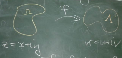
Theorem. If f is conformal and h is harmonic in \Lambda, then H is harmonic in \Omega where H(x,y) =h(u(x,y),v(x,y)).
Proof. Messy in general but straightforward when \Lambda is simply connected. See §115 (8 Ed §104). \square
Example: Take h(u,v) = e^{-v}\sin u which is harmonic on the upper half-plane. Define w = z^2 on \Omega, the first quadrant. Thus, w = u+iv where u = x^2 - y^2 and v = 2xy.
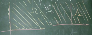
Applying this theorem, we know that H(x,y) = e^{-2xy} \sin (x^2-y^2) is harmonic on \Omega. Note that Dirichlet and Neumann boundary conditions are preserved under conformal transformations (more next lecture). \circ